Dual-BLDC Balancing Platform: Designing an Unstable Plant to Test Real-Time Control

Why build an unstable machine on purpose?
A tuning tool proven only in simulation proves very little. Simulation gives you clean signals, perfect timing and a plant that behaves exactly like its equations. I wanted the opposite: a system that falls the moment control stops, reacts within milliseconds, and brings every real-world problem with it: motor noise, actuator nonlinearity and limited computing power.
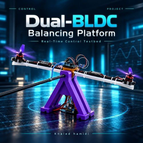
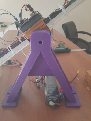
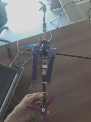
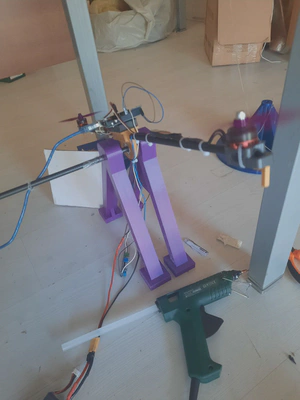
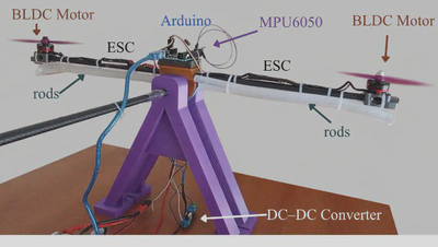
So I designed a dual-BLDC balancing platform: a rigid beam free to rotate around a central pivot, with a brushless motor and propeller at each end. It is the same problem as a classical inverted pendulum, and it emulates the pitch axis of a two-rotor UAV. If the controller is wrong, the beam slams into the ground. If it is right, the beam floats level on two columns of air.
This platform was the hardware validation plant for my online PID tuning & visualization tool.
Mechanical design
I modeled the whole assembly in Fusion 360 before printing a single part. Two requirements drove the design:
- Mass symmetry. If the two arms are not mirror images, gravity puts a constant torque on the beam and the controller has to fight a bias instead of balancing.
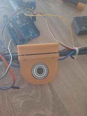
- A low-friction pivot. Friction at the pivot hides dynamics and makes the system look more stable than it really is. The pivot block carries a ball bearing, so the beam rotates freely in the pitch plane.
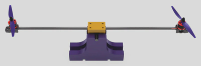
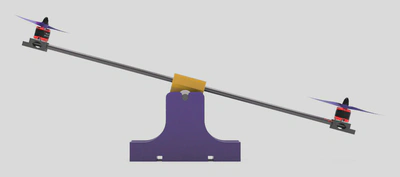
All structural parts were 3D-printed in PLA (25% infill, 0.2 mm layers), which gave me good geometric accuracy and repeatable mass on both sides.
Dynamics: what the controller is fighting
The state of the system is its tilt angle $\theta(t)$, measured from the equilibrium position ($\theta = 0$). Applying Newton’s second law for rotation about the pivot:
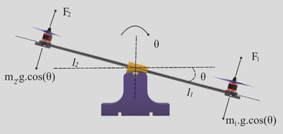
Here $m_1, m_2$ are the motor-assembly masses, $l_1, l_2$ their distances from the pivot, $F_1, F_2$ the propeller thrusts and $g$ the gravitational acceleration.
This is where the symmetric design pays off. With $m_1 = m_2 = m$ and $l_1 = l_2 = L$, the gravity terms cancel exactly:
$$ \ddot{\theta} = \frac{L\,(F_1 - F_2)}{2 m L^2} = \frac{F_1 - F_2}{2 m L} $$The beam’s acceleration depends only on the thrust difference. There is no restoring torque, so any small disturbance grows until active feedback stops it. Each propeller’s thrust follows the classic quadratic law:
$$ T = C_T \, \omega^2 $$where $C_T$ is the propeller thrust constant and $\omega$ the rotor speed. This quadratic relationship is a nonlinearity sitting directly between the controller output and the physical force.
Electronics & hardware architecture
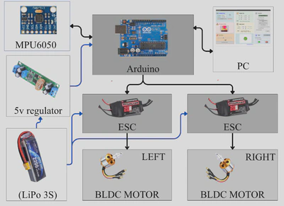
| Component | Role | Key specifications |
|---|---|---|
| EMAX RS2205 ×2 | BLDC motors | 2300 KV, fixed-pitch propellers |
| Hobbywing Skywalker 20 A ×2 | ESCs | PWM command, 1–2 ms pulse |
| MPU6050 | IMU (at the pivot) | 3-axis gyro + accelerometer, I²C @ 400 kHz |
| Arduino Uno | Main controller | ATmega328P @ 16 MHz, serial @ 115200 bps |
| Li-Po battery | Power | 3S, 11.1 V, 1800 mAh |
| DC–DC converter | Logic supply | 5 V, 2 A, isolates logic from motor noise |
| PLA (3D-printed) | Frame | 25% infill, 0.2 mm layer height |
The logic rail is fed through a dedicated 5 V DC–DC converter to keep the motors’ switching noise away from the microcontroller and the sensor. As the experiments showed, isolating the supply alone is not enough.
Embedded control: from raw IMU data to differential thrust
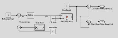
The Arduino runs a discrete control loop designed for 100 Hz ($T_s = 10$ ms). Each cycle runs the same pipeline: estimate → compare → compute → limit → mix.
1. Attitude estimation (complementary filter)
The gyroscope is fast but drifts. The accelerometer is drift-free but noisy. I fuse them with a complementary filter. The gyro rate is integrated:
$$ \theta_g[k] = \theta_g[k-1] + \dot{\theta}[k]\, T_s $$and blended with the accelerometer inclination $\theta_a[k]$, computed from $(a_x, a_y, a_z)$:
$$ \hat{\theta}[k] = \alpha \left( \hat{\theta}[k-1] + \dot{\theta}[k]\, T_s \right) + (1-\alpha)\, \theta_a[k], \qquad \alpha = 0.98 $$With $\alpha = 0.98$, the gyro dominates the fast dynamics and gravity slowly corrects the drift.
2. Discrete PID
With the tracking error $e[k] = \theta_{ref}[k] - \hat{\theta}[k]$:
$$ u[k] = K_p\, e[k] + K_i \sum_{i=0}^{k} e[i]\, T_s + K_d\, \frac{e[k] - e[k-1]}{T_s} $$3. Saturation
To protect the actuators and limit integral windup, the output is clamped to a symmetric limit $L$, the PID limit that can be set live from the tool:
$$ u'[k] = \begin{cases} +L, & u[k] > +L \\ u[k], & -L \le u[k] \le +L \\ -L, & u[k] < -L \end{cases} $$4. Differential mixing
Finally, the limited signal is split symmetrically around a neutral throttle $U_{base}$:
$$ PWM_1[k] = U_{base} - u'[k], \qquad PWM_2[k] = U_{base} + u'[k] $$One motor speeds up while the other slows down, so the net thrust stays roughly constant and the controller output becomes a pure torque command.
In firmware, the core loop is deliberately compact:
void loop() {
  unsigned long currentTime = millis();
  mpu.update();
  angle = mpu.getAngleY();

  if (pid.Compute() && !emergency) {
    int motor1 = constrain(baseSpeed - out, 1000, 2000);
    int motor2 = constrain(baseSpeed + out, 1000, 2000);
    ESC.writeMicroseconds(motor1);
    ESC2.writeMicroseconds(motor2);
  }

  if (currentTime - lastSerialTime >= SERIAL_INTERVAL) {
    handleSerialCommands();          // non-blocking, newline-terminated
    lastSerialTime = currentTime;
  }
}
Incoming commands are assembled character by character and applied atomically: a new gain goes through pid.SetTunings() and takes effect within one sampling period. Telemetry is rate-limited on its own timer so streaming data never takes over the loop. Tuned values are stored in EEPROM, so the platform boots with its last good configuration.
What the hardware taught me
This is the part I value most. The platform balanced, and the tool tuned it live. But the experiments also measured exactly why the balance was not perfectly smooth, and turned two hidden problems into numbers.
Finding 1: the loop wasn’t really running at 100 Hz
The firmware was designed for 100 Hz. The time-stamped logs showed an actual average loop period of about 30 ms, roughly 33 Hz. A single-core 8-bit ATmega328P has to run I²C sensor reads, the PID computation, two ESC updates and bidirectional serial communication sequentially in every cycle.
For inverted-pendulum-type systems, a common guideline is a minimum update rate of about 50 Hz for robust stability. At 33 Hz the platform still balanced, but with persistent low-amplitude oscillations: the controller simply couldn’t react fast enough to reject disturbances.
To separate communication cost from computation cost, I added a Visualization-Off mode that stops telemetry streaming. The response got noticeably smoother, which confirms that streaming adds load. The oscillation didn’t disappear, though, so the main bottleneck is the microcontroller itself, not the protocol.
Finding 2: the motors were poisoning the sensor
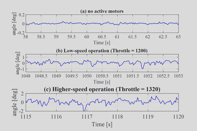
The second problem was electromagnetic interference. I recorded the steady-state angle in 5-second windows under three conditions:
| Condition | Std. deviation σ | Peak-to-peak |
|---|---|---|
| Motors off | 0.014° | 0.080° |
| Low speed (1200 µs) | 0.264° | 1.610° |
| Balancing speed (1320 µs) | 0.534° | 3.840° |
At balancing throttle, sensor noise rose 37 times in standard deviation and 48 times in peak-to-peak amplitude compared with the motors-off baseline. Noise growing with motor power points clearly at EMI from the BLDC motors and ESCs. For the controller this is critical: the derivative term reads high-frequency noise as real motion and issues corrections the beam never needed.
Where I’d take it next
- Move the controller to a faster 32-bit MCU to bring the real loop rate safely above 100 Hz.
- Harden the sensing chain against EMI: shielding, cable routing, sensor placement, and filtering on the measured angle.
- Use the logged data for system identification and model-based tuning, then compare it against manual tuning done with the tool.
Related posts in this series
- 💻 PID Tuning aVT: the open-source tuning tool: architecture, protocol and Software-in-the-Loop validation.
- 📄 Research publication in the Turkish Journal of Engineering: the peer-reviewed paper behind this work.