Time Response Analysis of RC and RLC Circuits: Understanding Signal Behavior
Introduction
When your phone rings, your router picks up a Wi-Fi signal, or a car’s control unit makes a split-second decision, a hidden phenomenon is at work: the response of electrical circuits to a sudden change in signal. This response determines a system’s speed, accuracy, and stability, and it’s what separates a reliable device from one that is unstable or slow.
Despite the complexity of modern electronics, the essence of this phenomenon can be explained through just three circuits: series RC, series RLC, and parallel RLC. These circuits are not just collections of components; they are the models upon which signal filters, communication circuits, power converters, control systems, and sensors are built. Understanding their time response is the first step to understanding how electrons interact with time and how waves are formed inside every device we use daily.
First: The RC Series Circuit — The School of Charging and Discharging
The Basic Idea
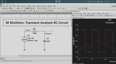
The RC circuit is the simplest model through which an engineer can understand how a circuit responds to any changing signal. The time constant,
$$ \tau = RC $$, is a direct indicator of how quickly the circuit reacts to the signal.
Simulation Analysis
- The input signal is a square wave (an instantaneous change).
- The output signal is curved due to the capacitor charging and discharging.
- This behavior represents a Low Pass Filter.
Real-World Uses
- Smoothing the output of DC converters
- Filtering noise from signals
- Time delay circuits
Second: The RLC Series Circuit — Damped Oscillation
The Basic Idea
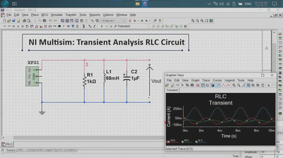
With both a capacitor and an inductor, the circuit begins to exchange electrical and magnetic energy. However, the presence of the resistor causes the oscillation to gradually decrease. The resonant frequency is:
$$ f_0 = \frac{1}{2\pi\sqrt{LC}} $$What Does the Simulation Show?
- A sinusoidal oscillation that starts large and then fades away.
- The current and voltage swing around an equilibrium point.
- Stability is gradually achieved due to the resistance.
Real-World Uses
- Selective frequency filters
- Radio receivers
- System stability analysis
Third: The RLC Parallel Circuit — Nearly Free Oscillation
The Basic Idea
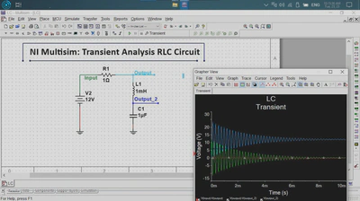
Connecting the components in parallel reduces the effect of resistance, allowing for a stronger and longer-lasting oscillation:
- More energy is exchanged between L and C
- A clear and stable frequency
- Very slow decay of the response
Simulation Results
- The oscillation has a higher amplitude than the series circuit.
- The waveform is purer.
- Damping is very weak.
Real-World Uses
This particular circuit is the heart of:
- Antennas
- RF Resonators
- Frequency amplification circuits
- RFID and NFC
Comprehensive Comparison
| Circuit | Behavior | Applications |
|---|---|---|
| RC Series | Exponential charge/discharge | Filters, Control, Power Conversion |
| RLC Series | Damped oscillation | Communications, Analysis, Filters |
| RLC Parallel | Nearly free oscillation | Antennas, RF, Resonant Systems |
Conclusion
These three circuits are not just laboratory exercises; they are fundamental to understanding how a signal oscillates, how a circuit stabilizes, and how systems behave during any sudden change. Using simulation tools like NI Multisim, these phenomena can be clearly visualized, providing insight into how all modern technologies are built.
